Eighteen Models, One Decision: Finding a Better Small Model for Linking Names to Wikidata

In the last post, our team at Yale linked 7.2 million people named in Europeana’s cultural heritage records to Wikidata. A small model read each record and its Wikidata candidates and decided which candidate was the person, or that none was. The model was GLiNER2.5-Decide, a 340-million-parameter classifier. Three copies of it, averaged, agreed with our reference labels 93.7% of the time.

That post ended with the model we had, not necessarily the best model we could have. GLiNER2.5-Decide was the first decision model we tried, and the field moves fast. In the past few weeks, a whole family of open models built for exactly this kind of question has appeared. So we asked the obvious question: if we trained every serious candidate the same way, on the same data, which one would make the best decisions?

We fine-tuned eighteen of them. The best, kev-4b, agrees with the labels 97.1% of the time and links only 4.1% of the people who have no match in Wikidata. GLiNER2.5-Decide, trained the same way, reaches 91.3% and links 20.7% of them. This post is about how we ran that comparison fairly, and what it taught us.

Some background, briefly

The task hasn’t changed. For each person in a catalogue, a search finds a short list of Wikidata candidates, everyone who might be meant. A model then reads the record and the candidates and decides: one of them, or none. The “none” answer matters as much as the links. A missing link costs you a link; a false link quietly merges two different people into one. (The last post explains why at length.)

Models that make this kind of decision are often called System One models, after the fast, intuitive kind of thinking in psychology. They don’t write prose. They take a text, which they call the state, and a typed question, and return a probability for every possible answer. There are three kinds of question:

Choice: pick one option from a list. Linking a person is a Choice: the options are the candidates plus “none.”
Score: rate the text on a scale, such as one to five.
Noul: is a statement true? For example, “the person in this record is this candidate.”

The format was popularised by Jev, a commercial model from TypeSafe that we compared against in the last post. In the weeks since, independent researchers have released open models that answer the same three kinds of question, most of them built by fine-tuning an open language model and attaching a small decision layer. Some are tiny encoders that run on a laptop; some are 27-billion-parameter models that need a data-centre GPU.

The same question, read five ways

What makes these models hard to compare is that they read a question in genuinely different ways. Give them the same record and the same three options, and each turns it into numbers differently:

Animated diagram. One decision, a record naming 'Boom BK' with two candidates and 'none', shown to five kinds of decision model: a label classifier that scores each option label; option-marker encoders that score a marker token placed before each option; decoders that list lettered options and read the next-token scores of the letters; a pointer head that compares each option's closing token with a final decide token; and models that write one prompt per option and ask whether it is correct. 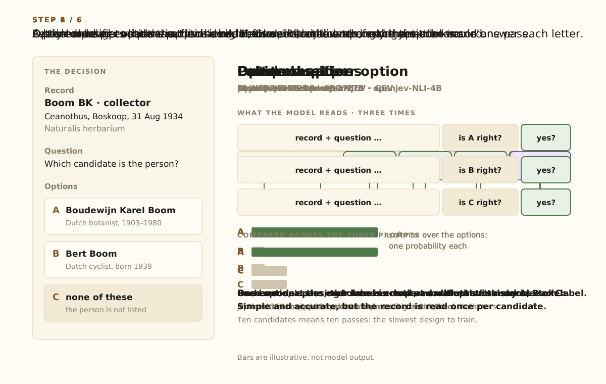— Five ways of reading the same decision. The bars are illustrative; the layouts are the ones each model was built with.

A label classifier (GLiNER2.5-Decide) treats the options as labels and scores each one against the text in a single pass.
Option-marker encoders (Laya, von, bekko) put a marker in front of each option and read a score off each marker.
Lettered prompts (plumb, JevK5, decider, and the slot-head models JEV and GEV) list the options as A, B, C and read how strongly the model would answer each letter.
A pointer head (the kev family) wraps each option in reserved tokens and compares the end of each option with a final “decide” token.
One prompt per option (Open-Jev, and an NLI model called openjev) asks “is this the right answer?” once for every candidate and compares the answers.

Each design comes with its own prompt layout, its own way of writing “none,” and its own idea of what a probability means. A fair comparison has to respect all of that, or it measures the wrapper instead of the model.

What we built

So we built a small training harness, system1-finetune-bench, which is on GitHub. It separates the three things that change between experiments:

The data. Any source is converted into one plain format: a state, a question type, the question, the options with their descriptions, and the answer. Adding a dataset is a short configuration file, not code.
How the question is asked. The same decision can be put to a model in different ways, for example with each candidate’s description next to the option or written into the record. We call these approaches, and they can be switched per experiment.
The model. Each architecture gets one adapter that knows how to build its native prompt and where to read its scores. Most of the eighteen models are a small configuration file on top of one of nine adapters.

Every run then follows the same recipe:

Score the untouched model on the test set, using its authors’ own prompt format and calibration (the zero-shot score).
Fine-tune it on the training set.
Keep the checkpoint that does best on a separate development set. The test set is never used for any choice.
Refit its confidence on the development set, so a probability of 0.9 means roughly nine in ten.
Score it on the test set again.

Every run is one job on Bouchet, Yale’s computing cluster. No outside model or API is called at any point.

The data is the one from the last post. We had labelled 4,000 Europeana persons with the help of a larger language model, of whom 3,456 had at least one candidate. Each of the eighteen models was trained on the same 2,780 decisions, chose its checkpoint on the same 312, and was tested on the same 364 held-out persons. Of those 364, 90 have no correct candidate. Because the last post taught us how much a single run can mislead, every model was trained three times with three different seeds, and we report the average.

One caution, as before. Every number below is agreement with labels that were produced with the help of a larger model and not checked by people. They are a strong reference, not ground truth.

Finding 1: GLiNER was the weakest choice we could have made

Animated chart. Agreement with the labels on 364 held-out persons, before and after fine-tuning, for eighteen models (mean of three seeds). After fine-tuning: kev-27b 97.4%, decider-35B-A3B 97.3%, kev-4b 97.1%, JEV-27B 96.9%, kev-9b 96.6%, Open-Jev-27B 96.5%, JEV-9B 96.1%, Open-Jev-9B 96.0%, JevK5-9B 95.8%, decider-4b 95.5%, GEV-26B 95.3%, openjev-NLI-4B 95.1%, decider-2b 94.4%, plumb-4b 94.4%, bekko-400m 93.0%, von 91.8%, Laya 91.6%, GLiNER2.5-Decide 91.3%. 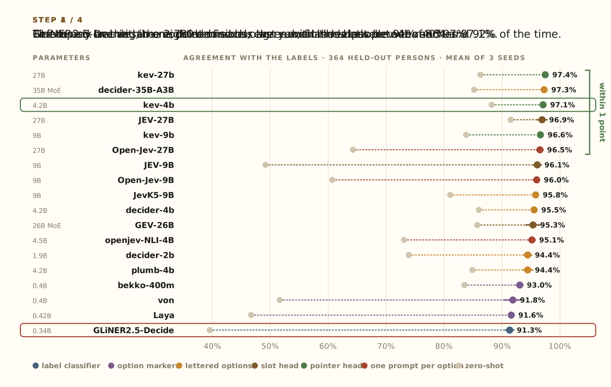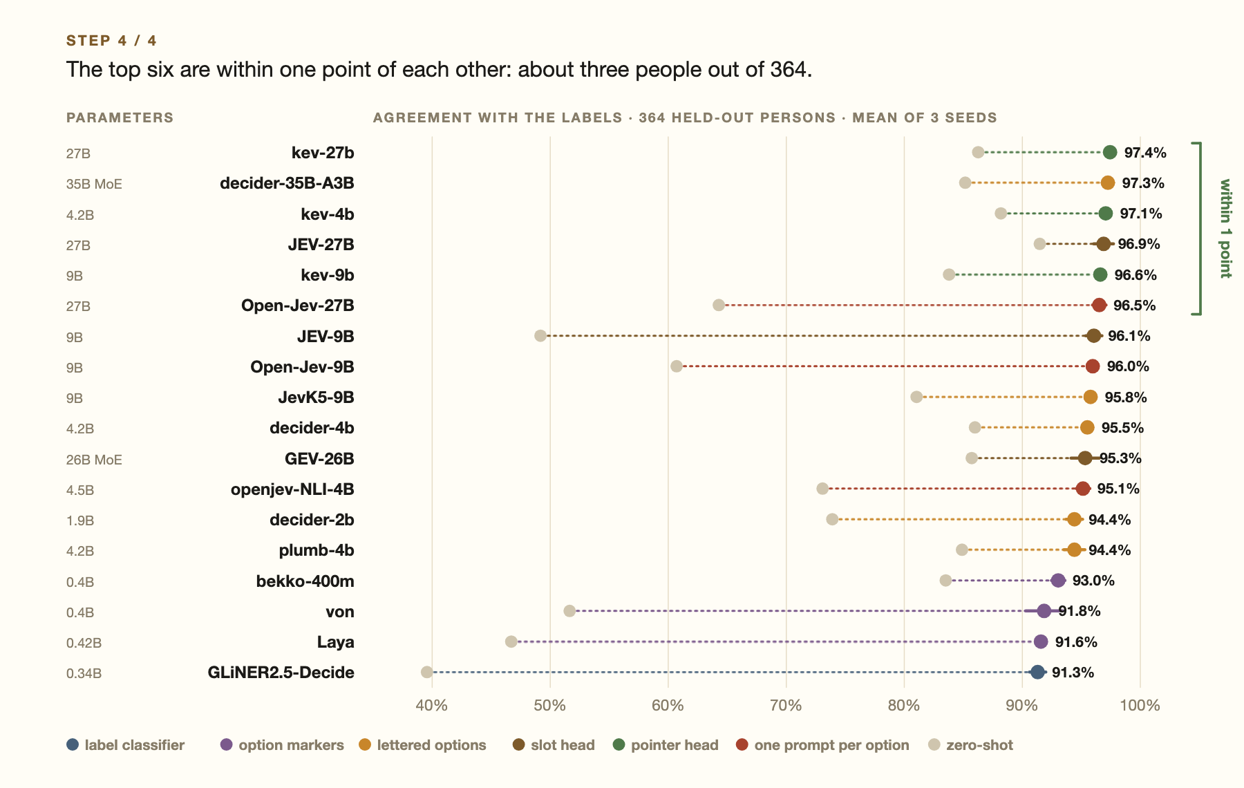— Grey: the untouched model. Coloured: after fine-tuning, with a short bar for the spread across three seeds. The colour shows how each model reads the options.

Before training, the models are all over the place. They agree with the labels anywhere from 40% (GLiNER2.5-Decide) to 92% (JEV-27B) of the time. Several of the open models are already good linkers out of the box: kev-4b gets 88% right without seeing a single Europeana example.

After training on the same 2,780 decisions, the spread collapses to 91–97%. And GLiNER2.5-Decide, the model behind the last post’s seven-million-name run, finishes last. It gains more than fifty points from fine-tuning and still trails every other model. Its 91.3% here is close to what we measured in the last post (91.8–93.4% for single copies), which is a useful check that the harness trains it properly. It lands a little lower because here it starts from the original release, not from our museum-terms model, and trains on slightly less data.

At the other end, kev-4b reaches 97.1% ± 0.3. That single model beats the average of three GLiNER copies from the last post (93.7%).

Finding 2: the better models are also more careful

Agreement counts every mistake the same way. For a catalogue, the costly mistake is the false link: attaching a record to a person who isn’t in it. It helps to see it directly.

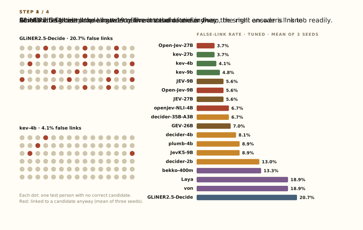
Animated chart. 90 of the 364 held-out persons have no correct candidate. GLiNER2.5-Decide links about 19 of them to someone anyway (20.7%); kev-4b about 4 (4.1%). False-link rates for all eighteen models range from 3.7% (Open-Jev-27B, kev-27b) to 20.7% (GLiNER2.5-Decide). — The false-link rate counts only the 90 test persons whose right answer is “none”: the share of them a model linked to someone anyway.

The false-link rate and agreement measure different things, so they don’t add up to anything. Agreement is over all 364 people. The false-link rate is over only the 90 who have no match: of those, how many did the model link anyway? GLiNER2.5-Decide links about 19 of the 90 to someone. kev-4b links about 4. That is the difference between one in five and one in twenty-five.

In the last post, getting GLiNER’s false links down to 6.7% took three models, a rule that all three must agree, and giving up some links. kev-4b gets lower, 4.1%, on its own, while still finding 97.4% of the links. The pattern holds across the chart. The larger decoders (kev, JEV, Open-Jev) are the cautious ones, and the small encoders link too readily.

A caveat: with only 90 such people, each false link moves the rate by more than a point, so these numbers wobble between seeds. kev-4b’s three runs made 6, 3 and 2 false links.

Finding 3: bigger stops paying at about four billion parameters

We tried the larger versions of the strongest families too, up to 35 billion parameters.

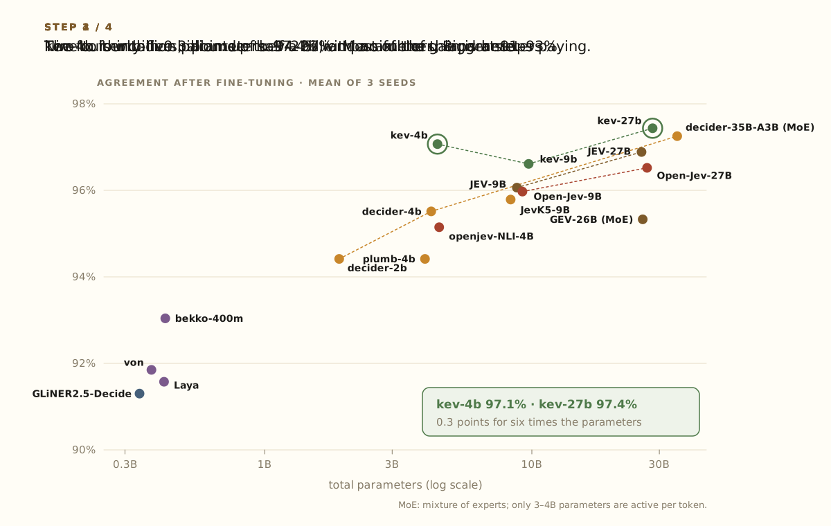
Animated scatter of agreement after fine-tuning against model size. Encoders under half a billion parameters reach 91–93%; models of two to four billion 94–97%; nine to thirty-five billion up to 97.4%. kev-4b (97.1%) is within 0.3 points of kev-27b (97.4%) with a sixth of the parameters. — Agreement after fine-tuning against total parameters, on a log scale. Dotted lines join sizes of the same family.

Most of the gain comes between half a billion and four billion parameters. Beyond that the curve is flat. kev-27b is the most accurate model we trained, at 97.4%, and the mixture-of-experts decider-35B-A3B is close behind at 97.3%. But kev-4b, with a sixth of kev-27b’s parameters, is only 0.3 points behind. That is about one person in 364, well inside the variation between seeds. The kev family isn’t even monotonic: kev-9b lands slightly below kev-4b.

The top six models are all within a point of each other: kev-27b, decider-35B-A3B, kev-4b, JEV-27B, kev-9b and Open-Jev-27B. On this test set, they are effectively tied. What the largest models do buy is a little consistency. kev-27b’s three runs are among the most consistent we saw, and it shares the lowest false-link rate (3.7%) with Open-Jev-27B.

The decider family is the clearest case of steady improvement with size: 94.4% at 2 billion parameters, 95.5% at 4 billion, 97.3% at 35 billion. Only 3 billion of decider-35B-A3B’s parameters are used for any one word, so it is cheaper to run than its size suggests.

Finding 4: how you ask matters before training, much less after

The harness lets us change how a question is put to a model without changing the model. We tried this on the first ten models, with one run per combination. These are single runs, and the same model trained twice can differ by up to three points, so small gaps here mean nothing.

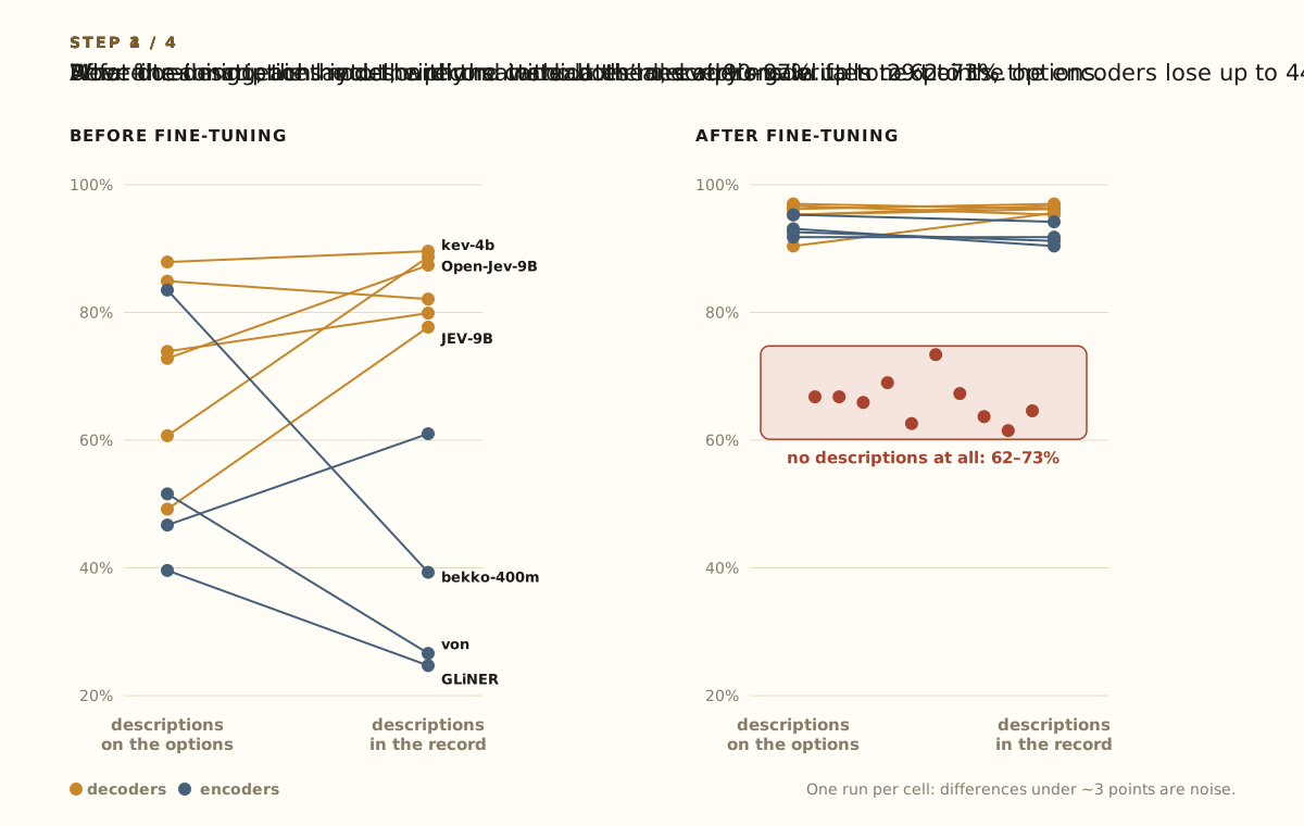
Animated slope chart for ten models. Before fine-tuning, moving the candidate descriptions from the options into the record raises the decoders (JEV-9B 49% to 78%, Open-Jev-9B 61% to 89%) and lowers the encoders (bekko 84% to 39%, von 52% to 27%, GLiNER 40% to 25%). After fine-tuning both layouts reach 90–97%. With no descriptions at all, every model falls to 62–73% even after fine-tuning. — Each line is one model. Left: untouched. Right: after fine-tuning. Orange lines are decoders, blue lines encoders.

Three things stand out:

The descriptions are what make it work. Each candidate comes with a one-line description from Wikidata, such as Dutch botanist (1903–1980). Take the descriptions away and leave only the identifiers, and every model falls to 62–73%, even after training.
Where you put them matters a lot, until you train. For an untouched model, writing the descriptions into the record instead of next to the options lifts the decoders by up to 29 points (JEV-9B from 49% to 78%, Open-Jev-9B from 61% to 89%). It sinks the encoders by up to 44 (bekko from 84% to 39%). If you use these models off the shelf, match the layout to the architecture.
After fine-tuning, layout barely matters. Both layouts land at 90–97%, and so does relabelling the options A, B, C. Training teaches the model whatever layout you give it.

We also tried the other two question types. For the yes/no version of the task (“is this candidate the person?”), the large decoders reach 95–98% after training, with JEV-9B the best at 98.4%. For scores on a five-level sentiment scale, describing what each level means helps an untouched model a great deal. Without the descriptions, the larger models’ average error grows by up to three quarters. After training, the differences shrink to almost nothing.

A note on time and memory

The obvious next question is cost.

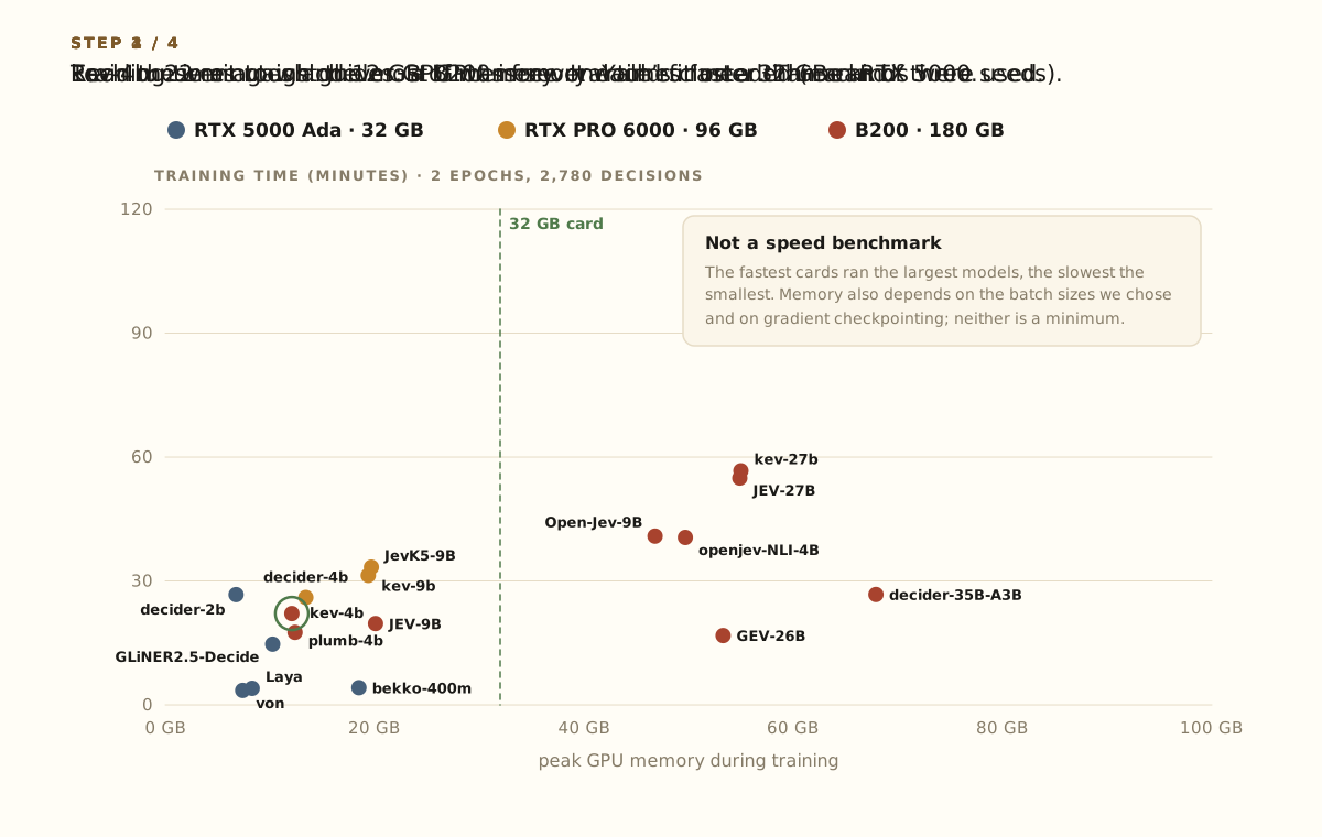
Animated scatter of training time against peak GPU memory for the eighteen fine-tunes, coloured by the GPU each ran on: RTX 5000 Ada (32 GB), RTX PRO 6000 (96 GB) or B200 (180 GB). kev-4b took 22 minutes and 12 GB on a B200; Open-Jev-27B 108 minutes and 94 GB. Times and memory depend on the GPU and on our batch settings, so they are rough guides, not benchmarks. — Training time against peak GPU memory, mean of three seeds, coloured by the GPU each run happened to get.

Please read this chart as a rough guide, not a benchmark. Each job ran on whichever GPU was free on the cluster at the time. We used three kinds of card, and they differ a lot in speed: an NVIDIA RTX 5000 Ada (32 GB), an RTX PRO 6000 (96 GB), and a B200 (180 GB), which is several times faster than the RTX 5000.

As it happened, the four small encoders all trained on the slowest card, and most of the large models trained on the fastest. That makes the large models look cheaper next to the small ones than they really are. The times also include the regular checks on the development set during training.

Peak memory is the most GPU memory each run used. It depends on the batch sizes we chose and on a memory-saving technique (gradient checkpointing) we turned on, so it is what our settings needed, not the least the model could run in. A different card, batch size or sequence length would give different numbers for every model.

With that said, the order of magnitude is informative. The encoders train in minutes, on almost anything. kev-4b took 22 minutes and 12 GB on a B200, small enough to fit on a 32 GB card. The 27-billion-parameter models needed 55–94 GB and up to almost two hours, which means a data-centre card. Open-Jev-27B is the most expensive by far, because it reads the record once for every candidate.

What this means for us

kev-4b is the model we would use now. It matches the largest models to within the noise, it is markedly more cautious than GLiNER2.5-Decide, and it is small enough to train and run on the GPUs a university already has. Its confidence is also well calibrated after the refit (an expected calibration error of 0.014), which matters when you decide which links to trust and which to send for review. Our fine-tuned kev-4b is on Hugging Face, in kev’s own format, so kev’s server loads it directly. Reloaded from those files, it reproduces its test scores exactly.

One run is still not a result. Across eighteen models, three seeds each, the spread between identical runs of the same model was often as large as the gap between neighbouring models. A 3-point difference from a single run, which is what we often see reported, can be pure chance.

Fine-tuning is the great equaliser. Untouched, these models range from 40% to 92% on our task, and their rankings change with the prompt layout. Trained on 2,780 examples, they land within six points of each other, and the layout hardly matters. If you have a few thousand labelled decisions, the choice of model matters less than you might think, as long as you avoid the weakest designs.

Some limits remain:

One task, one test set. Everything here is person reconciliation against Wikidata in Europeana records, with 364 test persons. The ranking might be different for places, subjects or other catalogues.
The labels are not the truth. Agreement with a larger model’s labels is a proxy, and above about 95% we are partly measuring that model’s own mistakes, as we saw in the last post.
Licences vary. Most of these models are Apache-2.0 or MIT. bekko-400m has no licence declared yet, so it is fine to experiment with but not to build on.
The full run hasn’t been redone. The seven million links from the last post still come from GLiNER2.5-Decide. Re-running them with kev-4b is the obvious next step.

Every model, every seed and every prompt variant went through the same pipeline and the same splits. That is what makes these numbers comparable. And it means the next decision model that appears is one configuration file and one overnight run away from a place on this chart. The harness, the configurations for all eighteen models and the full results are on GitHub.